Function Reference: qsmmm
- Function File: [U, R, Q, X, p0, pm] = qsmmm (lambda, mu)
- Function File: [U, R, Q, X, p0, pm] = qsmmm (lambda, mu, m)
- Function File: pk = qsmmm (lambda, mu, m, k)
Compute utilization, response time, average number of requests in service and throughput for a queue, a queueing system with identical servers connected to a single FCFS queue.
$$ \pi_k = \cases{ \displaystyle{\pi_0 { ( m\rho )^k \over k!}} & $0 \leq k \leq m$;\cr\cr \displaystyle{\pi_0 { \rho^k m^m \over m!}} & $k>m$.\cr } $$$$ \pi_0 = \left[ \sum_{k=0}^{m-1} { (m\rho)^k \over k! } + { (m\rho)^m \over m!} {1 \over 1-\rho} \right]^{-1} $$
INPUTS
-
lambda
Arrival rate (lambda>0).
mu Service rate (mu>lambda).
m Number of servers (m ≥ 1).
Default is m=1.
k Number of requests in the system (k ≥ 0).
OUTPUTS
-
U
Service center utilization, .
RService center mean response time
QAverage number of requests in the system
X Service center throughput. If the system is ergodic,
we will always have X = lambda
p0Steady-state probability that there are 0 requests in the system
pmSteady-state probability that an arriving request has to wait in the queue
pkSteady-state probability that there are k requests in the system (including the one being served).
If this function is called with less than four parameters, lambda, mu and m can be vectors of the same size. In this case, the results will be vectors as well.
REFERENCES
- G. Bolch, S. Greiner, H. de Meer and K. Trivedi, Queueing Networks and Markov Chains: Modeling and Performance Evaluation with Computer Science Applications, Wiley, 1998, Section 6.5
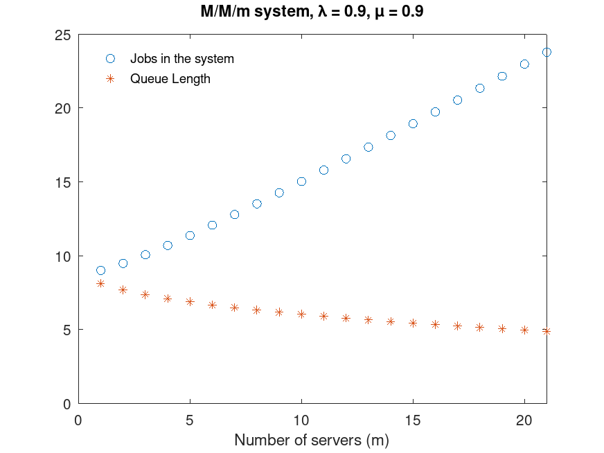
Example: 1
 # This is figure 6.4 on p. 220 Bolch et al.
 rho = 0.9;
 ntics = 21;
 lambda = 0.9;
 m = linspace(1,ntics,ntics);
 mu = lambda./(rho .* m);
 [U R Q X] = qsmmm(lambda, mu, m);
 qlen = X.*(R-1./mu);
 plot(m,Q,"o",qlen,"*");
 axis([0,ntics,0,25]);
 legend("Jobs in the system","Queue Length","location","northwest");
 legend("boxoff");
 xlabel("Number of servers (m)");
 title("M/M/m system, \\lambda = 0.9, \\mu = 0.9");
|
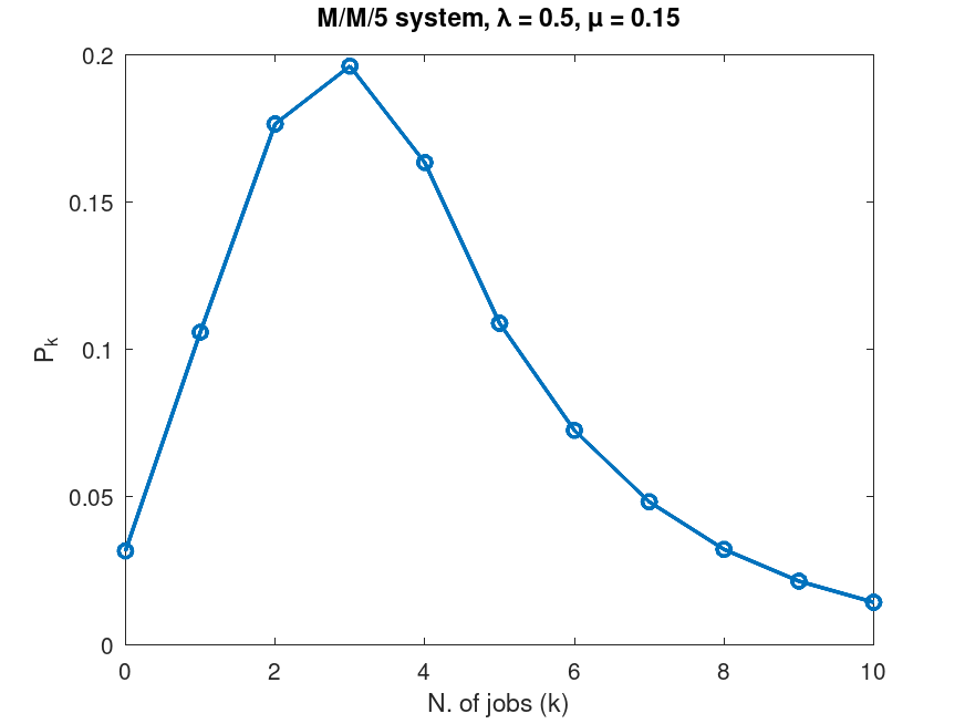
Example: 2
 ## Given a M/M/m queue, compute the steady-state probability pk of
 ## having k jobs in the systen.
 lambda = 0.5;
 mu = 0.15;
 m = 5;
 k = 0:10;
 pk = qsmmm(lambda, mu, m, k);
 plot(k, pk, "-o", "linewidth", 2);
 xlabel("N. of jobs (k)");
 ylabel("P_k");
 title(sprintf("M/M/%d system, \\lambda = %g, \\mu = %g", m, lambda, mu));
|
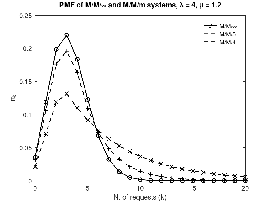
Example: 3
 ## This code produces Fig. 4 from the paper: M. Marzolla, "A GNU
 ## Octave package for Queueing Networks and Markov Chains analysis",
 ## submitted to the ACM Transactions on Mathematical Software.

 lambda = 4; mu = 1.2;
 k = 0:20;
 pk_inf = qsmminf(lambda, mu, k);
 pk_4 = qsmmm(lambda, mu, 4, k);
 pk_5 = qsmmm(lambda, mu, 5, k);

 plot(k, pk_inf, "-ok;M/M/\\infty;", "linewidth", 1.5, ...
      k, pk_5, "--+k;M/M/5;", "linewidth", 1.5, ...
      k, pk_4, "--xk;M/M/4;", "linewidth", 1.5 ...
     );
 xlabel("N. of requests (k)");
 ylabel("\\pi_k");
 legend("boxoff");
 title(sprintf("PMF of M/M/\\infty and M/M/m systems, \\lambda = %g, \\mu = %g", lambda, mu));
|