Function Reference: qncmmva
- Function File: [U, R, Q, X] = qncmmva (N, S )
- Function File: [U, R, Q, X] = qncmmva (N, S, V)
- Function File: [U, R, Q, X] = qncmmva (N, S, V, m)
- Function File: [U, R, Q, X] = qncmmva (N, S, V, m, Z)
- Function File: [U, R, Q, X] = qncmmva (N, S, P)
- Function File: [U, R, Q, X] = qncmmva (N, S, P, r)
- Function File: [U, R, Q, X] = qncmmva (N, S, P, r, m)
Compute steady-state performance measures for closed, multiclass queueing networks using the Mean Value Analysys (MVA) algorithm.
Queueing policies at service centers can be any of the following:
- FCFS
(First-Come-First-Served) customers are served in order of arrival; multiple servers are allowed. For this kind of queueing discipline, average service times must be class-independent.
(Processor Sharing) customers are served in parallel by a single server, each customer receiving an equal share of the service rate.
(Last-Come-First-Served, Preemptive Resume) customers are served in reverse order of arrival by a single server and the last arrival preempts the customer in service who will later resume service at the point of interruption.
(Infinite Server) customers are delayed independently of other customers at the service center (there is effectively an infinite number of servers).
INPUTS
-
N(c)
number of class requests; N(c) ≥ 0. If
class has no requests (N(c) == 0), then for
all k, this function returns
U(c,k) = R(c,k) = Q(c,k) = X(c,k) = 0
S(c,k) mean service time for class requests at center
(S(c,k) ≥ 0). If the service time at center
is class-dependent, then center is assumed
to be of type –PS (Processor Sharing). If center
is a FCFS node (m(k)>1), then the service
times must be class-independent, i.e., all classes
must have the same service time.
V(c,k) average number of visits of class requests at
center ; V(c,k) ≥ 0, default is 1.
If you pass this argument, class switching is not allowed
P(r,i,s,j) probability that a class request completing service at center
is routed to center as a class request; the
reference stations for each class are specified with the paramter
r. If you pass argument P, class switching is
allowed; however, you can not specify any external delay (i.e.,
Z must be zero) and all servers must be fixed-rate or
infinite-server nodes (m(k) ≤ 1 for all
).
r(c) reference station for class . If omitted, station 1 is the
reference station for all classes. See qncmvisits.
m(k) If m(k)<1, then center is assumed to be a delay
center (IS node ). If m(k)==1, then
service center is a regular queueing center
(–FCFS, –LCFS-PR or –PS).
Finally, if m(k)>1, center is a
–FCFS center with m(k) identical servers.
Default is m(k)=1 for each .
Z(c) class external delay (think time); Z(c) ≥
0. Default is 0. This parameter can not be used if you pass a
routing matrix as the second parameter of qncmmva.
OUTPUTS
-
U(c,k)
If is a FCFS, LCFS-PR or PS node (m(k) ≥
1), then U(c,k) is the class utilization at
center , . If is an
IS node, then U(c,k) is the class at center , defined as U(c,k) =
X(c,k)*S(c,k). In this case the value of
U(c,k) may be greater than one.
R(c,k) class response time at center . The class
at center is R(c,k) *
C(c,k). The total class system response time is
dot(R, V, 2).
Q(c,k) average number of class requests at center . The
total number of requests at center is
sum(Q(:,k)). The total number of class
requests in the system is sum(Q(c,:)).
X(c,k) class throughput at center . The class
throughput can be computed as X(c,1) / V(c,1).
NOTES
If the function call specifies the visit ratios V, then class switching is not allowed. If the function call specifies the routing probability matrix P, then class switching is allowed; however, in this case all nodes are restricted to be fixed rate servers or delay centers: multiple-server and general load-dependent centers are not supported.
In presence of load-dependent servers (e.g., if m(i)>1
for some ), the MVA algorithm is known to be numerically
unstable. Generally this problem shows up as negative values for the
computed response times or utilizations. This is not a problem with the
queueing package, but with the MVA algorithm;
as such, there is no known workaround at the moment (aoart from using a
different solution technique, if available). This function prints a
warning if it detects numerical problems; you can disable the warning
with the command warning("off", "qn:numerical-instability").
Given a network with service centers, job classes
and population vector , the MVA
algorithm requires space . The time
complexity is . This implementation is
slightly more space-efficient (see details in the code). While the
space requirement can be mitigated by using some optimizations, the
time complexity can not. If you need to analyze large closed networks
you should consider the qncmmvaap function, which implements
the approximate MVA algorithm. Note however that qncmmvaap
will only provide approximate results.
REFERENCES
- M. Reiser and S. S. Lavenberg, Mean-Value Analysis of Closed Multichain Queuing Networks, Journal of the ACM, vol. 27, n. 2, April 1980, pp. 313–322. 10.1145/322186.322195
This implementation is based on G. Bolch, S. Greiner, H. de Meer and K. Trivedi, Queueing Networks and Markov Chains: Modeling and Performance Evaluation with Computer Science Applications, Wiley, 1998 and Edward D. Lazowska, John Zahorjan, G. Scott Graham, and Kenneth C. Sevcik, Quantitative System Performance: Computer System Analysis Using Queueing Network Models, Prentice Hall, 1984. http://www.cs.washington.edu/homes/lazowska/qsp/. In particular, see section 7.4.2.1 ("Exact Solution Techniques").
See also: qnclosed, qncmmvaapprox, qncmvisits
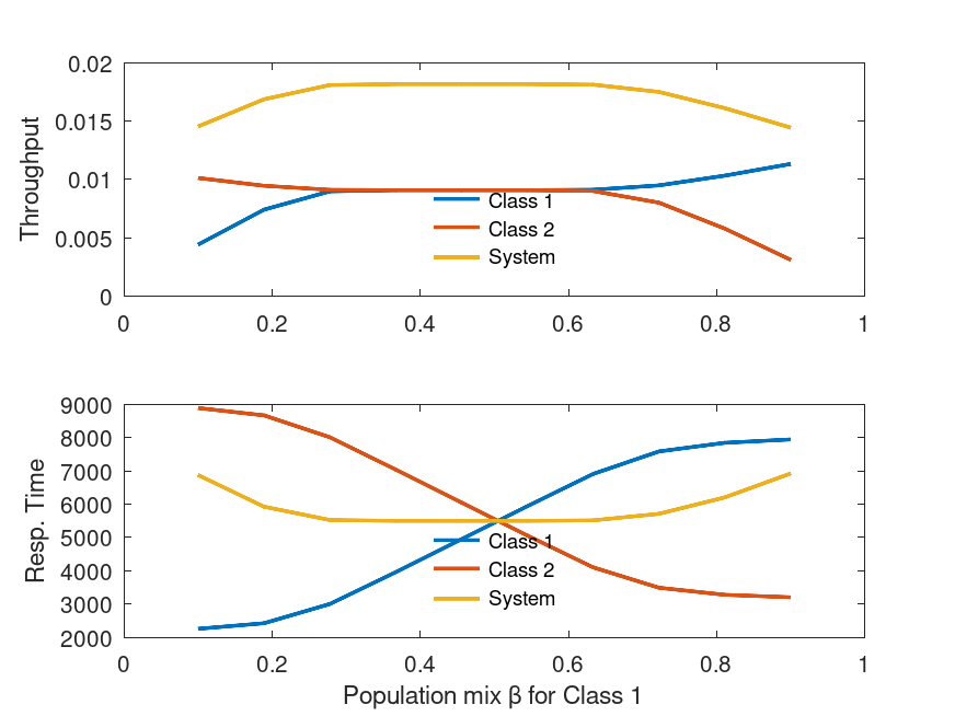
Example: 1
 Ntot = 100; # total population size
 b = linspace(0.1,0.9,10); # fractions of class-1 requests
 S = [20 80 31 14 23 12; ...
      90 30 33 20 14 7];
 V = ones(size(S));
 X1 = X1 = XX = zeros(size(b));
 R1 = R2 = RR = zeros(size(b));
 for i=1:length(b)
   N = [fix(b(i)*Ntot) Ntot-fix(b(i)*Ntot)];
   # printf("[%3d %3d]\n", N(1), N(2) );
   [U R Q X] = qncmmva( N, S, V );
   X1(i) = X(1,1) / V(1,1);
   X2(i) = X(2,1) / V(2,1);
   XX(i) = X1(i) + X2(i);
   R1(i) = dot(R(1,:), V(1,:));
   R2(i) = dot(R(2,:), V(2,:));
   RR(i) = Ntot / XX(i);
 endfor
 subplot(2,1,1);
 plot(b, X1, ";Class 1;", "linewidth", 2, ...
      b, X2, ";Class 2;", "linewidth", 2, ...
      b, XX, ";System;", "linewidth", 2 );
 legend("location","south"); legend("boxoff");
 ylabel("Throughput");
 subplot(2,1,2);
 plot(b, R1, ";Class 1;", "linewidth", 2, ...
      b, R2, ";Class 2;", "linewidth", 2, ...
      b, RR, ";System;", "linewidth", 2 );
 legend("location","south"); legend("boxoff");
 xlabel("Population mix \\beta for Class 1");
 ylabel("Resp. Time");
|
Example: 2
 S = [1 0 .025; 0 15 .5];
 P = zeros(2,3,2,3);
 P(1,1,1,3) = P(1,3,1,1) = 1;
 P(2,2,2,3) = P(2,3,2,2) = 1;
 V = qncmvisits(P,[3 3]); # reference station is station 3
 N = [15 5];
 m = [-1 -1 1];
 [U R Q X] = qncmmva(N,S,V,m)

U =

   14.3231         0    0.3581
         0    4.7070    0.1569

R =

    1.0000         0    0.0473
         0   15.0000    0.9337

Q =

   14.3231         0    0.6769
         0    4.7070    0.2930

X =

   14.3231         0   14.3231
         0    0.3138    0.3138
|
Example: 3
 C = 2; K = 3;
 S = [.01 .07 .10; ...
      .05 .07 .10 ];
 P = zeros(C,K,C,K);
 P(1,1,1,2) = .7; P(1,1,1,3) = .2; P(1,1,2,1) = .1;
 P(2,1,2,2) = .3; P(2,1,2,3) = .5; P(2,1,1,1) = .2;
 P(1,2,1,1) = P(2,2,2,1) = 1;
 P(1,3,1,1) = P(2,3,2,1) = 1;
 N = [3 0];
 [U R Q X] = qncmmva(N, S, P)

U =

   0.1261   0.6178   0.2522
   0.3152   0.1324   0.3152

R =

   0.014653   0.133148   0.163256
   0.073266   0.133148   0.163256

Q =

   0.1848   1.1752   0.4117
   0.4619   0.2518   0.5146

X =

   12.6089    8.8262    2.5218
    6.3044    1.8913    3.1522
|
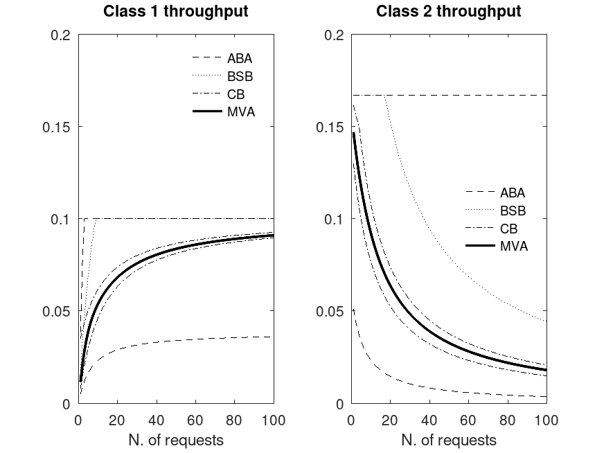
Example: 4
 S = [10 7 5 4;
      5  2 4 6];
 NN = 100;
 Xl_aba = Xu_aba = Xl_bsb = Xu_bsb = Xl_cb = Xu_cb = Xmva = Rmva = zeros(NN,2);
 for n=1:NN
   N=[n,10];
   [a b] = qncmaba(N,S);
   Xl_aba(n,:) = a; Xu_aba(n,:) = b;
   [a b] = qncmbsb(N,S);
   Xl_bsb(n,:) = a; Xu_bsb(n,:) = b;
   [a b] = qncmcb(N,S);
   Xl_cb(n,:) = a; Xu_cb(n,:) = b;
   [U R Q X] = qncmmva(N,S,ones(size(S)));
   Xmva(n,:) = X(:,1)';
 endfor
 subplot(1,2,1);
 plot(1:NN, Xl_aba(:,1), "--k",
      1:NN, Xu_aba(:,1), "--k;ABA;",
      1:NN, Xu_bsb(:,1), ":k;BSB;",
      1:NN, Xl_cb(:,1), "-.k",
      1:NN, Xu_cb(:,1), "-.k;CB;",
      1:NN, Xmva(:,1), "k;MVA;", "linewidth", 2);
 xlabel("N. of requests");
 ylim([0, 0.2]);
 title("Class 1 throughput"); legend("boxoff");
 subplot(1,2,2);
 plot(1:NN, Xl_aba(:,2), "--k",
      1:NN, Xu_aba(:,2), "--k;ABA;",
      1:NN, Xu_bsb(:,2), ":k;BSB;",
      1:NN, Xl_cb(:,2), "-.k",
      1:NN, Xu_cb(:,2), "-.k;CB;",
      1:NN, Xmva(:,2), "-k;MVA;", "linewidth", 2);
 xlabel("N. of requests");
 ylim([0, 0.2]);
 title("Class 2 throughput");
 legend("boxoff");
 legend("location", "east");
|