Function Reference: ctmcexps
- Function File: L = ctmcexps (Q, t, p )
- Function File: L = ctmcexps (Q, p)
With three arguments, compute the expected times L(i)
spent in each state during the time interval ,
assuming that the initial occupancy vector is p. With two
arguments, compute the expected time L(i) spent in each
transient state until absorption.
Note: In its current implementation, this function requires that an absorbing state is reachable from any non-absorbing state of .
INPUTS
-
Q(i,j)
infinitesimal generator matrix. Q(i,j)
is the transition rate from state to state ,
, .
The matrix Q must also satisfy the
condition for every .
tIf given, compute the expected sojourn times in
p(i) Initial occupancy probability vector; p(i) is the
probability the system is in state at time 0,
OUTPUTS
-
L(i)
If this function is called with three arguments, L(i) is
the expected time spent in state during the interval
. If this function is called with two arguments
L(i) is the expected time spent in transient state
until absorption; if state is absorbing,
L(i) is zero.
See also: dtmcexps
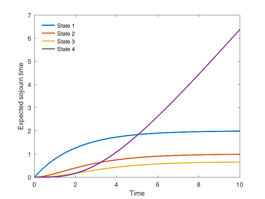
Example: 1
 lambda = 0.5;
 N = 4;
 b = lambda*[1:N-1];
 d = zeros(size(b));
 Q = ctmcbd(b,d);
 t = linspace(0,10,100);
 p0 = zeros(1,N); p0(1)=1;
 L = zeros(length(t),N);
 for i=1:length(t)
   L(i,:) = ctmcexps(Q,t(i),p0);
 endfor
 plot( t, L(:,1), ";State 1;", "linewidth", 2, ...
       t, L(:,2), ";State 2;", "linewidth", 2, ...
       t, L(:,3), ";State 3;", "linewidth", 2, ...
       t, L(:,4), ";State 4;", "linewidth", 2 );
 legend("location","northwest"); legend("boxoff");
 xlabel("Time");
 ylabel("Expected sojourn time");
|
Example: 2
 lambda = 0.5;
 N = 4;
 b = lambda*[1:N-1];
 d = zeros(size(b));
 Q = ctmcbd(b,d);
 p0 = zeros(1,N); p0(1)=1;
 L = ctmcexps(Q,p0);
 disp(L);

   2.0000   1.0000   0.6667        0
|