Function Reference: ctmc
- Function File: p = ctmc (Q)
- Function File: p = ctmc (Q, t, p0)
Compute stationary or transient state occupancy probabilities for a continuous-time Markov chain.
With a single argument, compute the stationary state occupancy probabilities for a continuous-time Markov chain with finite state space and infinitesimal generator matrix Q. With three arguments, compute the state occupancy probabilities that the system is in state at time t, given initial state occupancy probabilities at time 0.
INPUTS
-
Q(i,j)
Infinitesimal generator matrix. Q is a square
matrix where Q(i,j) is the transition rate from state
to state , for .
Q must satisfy the property that
tTime at which to compute the transient probability (). If omitted, the function computes the steady state occupancy probability vector.
p0(i)probability that the system is in state at time 0.
OUTPUTS
-
p(i)
If this function is invoked with a single argument, p(i)
is the steady-state probability that the system is in state ,
. If this function is invoked with three
arguments, p(i) is the probability that the system is in
state at time t, given the initial occupancy
probabilities p0(1), …, p0(N).
See also: dtmc
Example: 1
 Q = [ -1  1; ...
        1 -1  ];
 q = ctmc(Q)

q =

   0.5000   0.5000
|
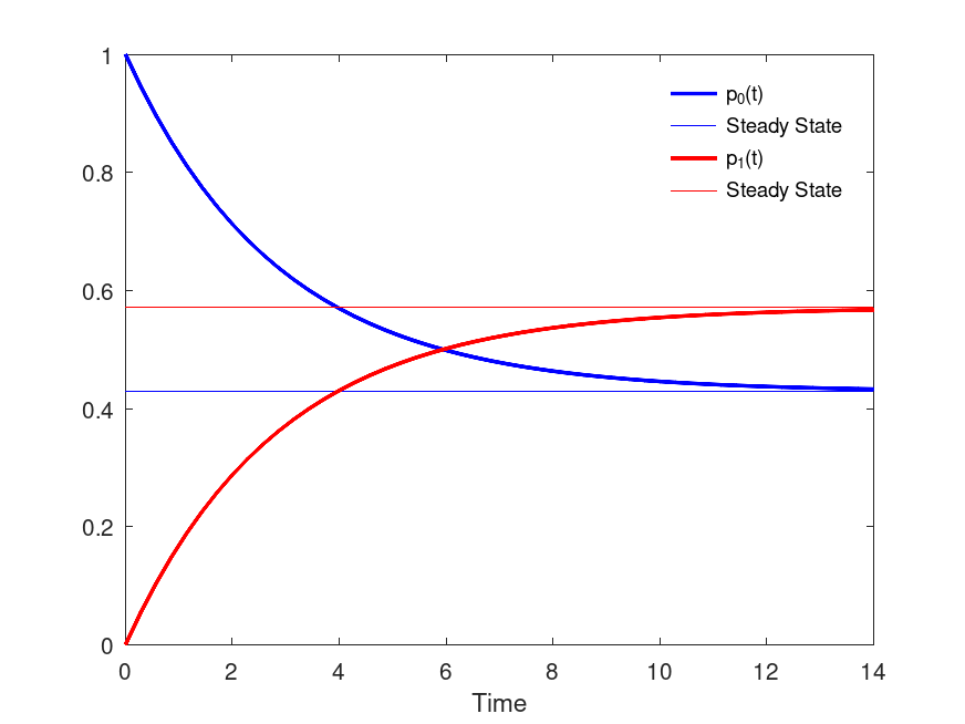
Example: 2
 a = 0.2;
 b = 0.15;
 Q = [ -a a; b -b];
 T = linspace(0,14,50);
 pp = zeros(2,length(T));
 for i=1:length(T)
   pp(:,i) = ctmc(Q,T(i),[1 0]);
 endfor
 ss = ctmc(Q); # compute steady state probabilities
 plot( T, pp(1,:), "b;p_0(t);", "linewidth", 2, ...
       T, ss(1)*ones(size(T)), "b;Steady State;", ...
       T, pp(2,:), "r;p_1(t);", "linewidth", 2, ...
       T, ss(2)*ones(size(T)), "r;Steady State;" );
 xlabel("Time");
 legend("boxoff");
|
Example: 3
 ##
 ## The code below is used in the paper: "M. Marzolla,
 ## "A GNU Octave package for Queueing Networks and Markov Chains analysis"
 ## (submitted to the ACM Transactions on Mathematical Software)
 ## to analyze the reliability model from Figure 2. The model
 ## has been originally described in the paper:
 ##
 ## David I. Heimann, Nitin Mittal, Kishor S. Trivedi, "Availability
 ## and Reliability Modeling for Computer Systems",
 ## Marshall C. Yovits (Ed.), Advances in Computers, Elsevier, Volume 31,
 ## 1990, Pages 175-233, ISSN 0065-2458, ISBN 9780120121311, DOI
 ## https://doi.org/10.1016/S0065-2458(08)60154-0. sep 1989, section
 ## 2.5.

 mm = 60; hh = 60*mm; dd = 24*hh; yy = 365*dd;
 a = 1/(10*mm);    # 1/a = duration of reboot (10 min)
 b = 1/30;         # 1/b = reconfiguration time (30 sec)
 g = 1/(5000*hh);  # 1/g = processor MTTF (5000 h)
 d = 1/(4*hh);     # 1/d = processor MTTR (4 h)
 c = 0.9;          # recovery probability
 [TWO,RC,RB,ONE,ZERO] = deal(1,2,3,4,5);
 ##      2    RC      RB        1     0
 Q = [ -2*g  2*c*g 2*(1-c)*g    0     0; ...  # 2
         0    -b       0        b     0; ...  # RC
         0     0      -a        a     0; ...  # RB
         d     0       0     -(g+d)   g; ...  # 1
         0     0       0        d    -d];     # 0
 p = ctmc(Q);

 disp("minutes/year spent in RC");
 p(RC)*yy/mm  # minutes/year spent in RC
 disp("minutes/year spent in RB");
 p(RB)*yy/mm  # minutes/year spent in RB
 disp("minutes/year spent in 0");
 p(ZERO)*yy/mm  # minutes/year spent in 0

 Q(ZERO,:) = Q(RB,:) = 0; # make states {0, RB} absorbing
 p0 = [ 1 0 0 0 0 ] ; # initial state occupancy probabiliies
 disp("MTBF (years)");
 MTBF = ctmcmtta(Q, p0) / yy # MTBF (years)

minutes/year spent in RC
ans = 1.5743
minutes/year spent in RB
ans = 3.4984
minutes/year spent in 0
ans = 0.6717
MTBF (years)
MTBF = 2.8376
|